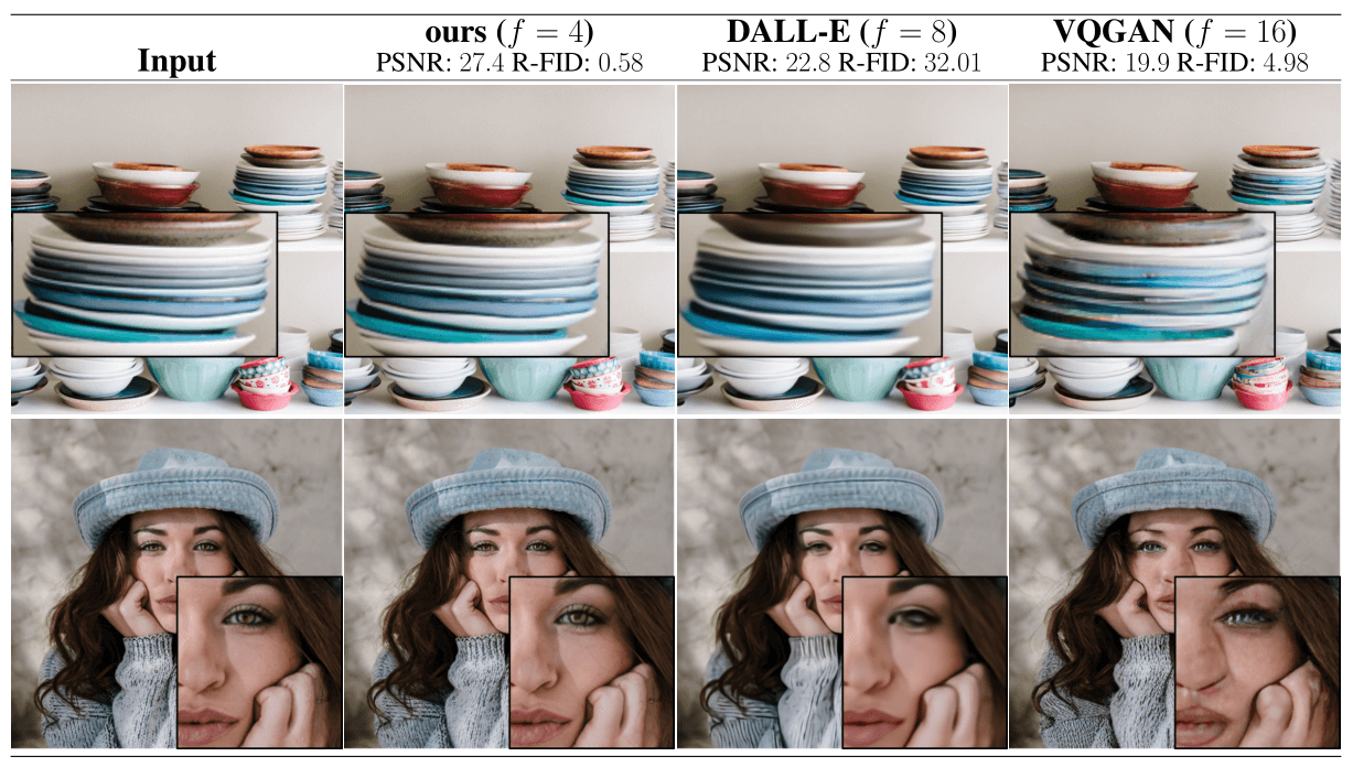
Figure 1. Boosting the upper bound on achievable quality with less agressive downsampling. Since diffusion models offer excellent inductive biases for spatial data, we do not need the heavy spatial downsampling of related generative models in latent space, but can still greatly reduce the dimensionality of the data via suitable autoencoding models, see Sec. 3. Images are from the DIV2K [1] validation set, evaluated at 5122 px. We denote the spatial downsampling factor by f . Reconstruction FIDs [26] and PSNR are calculated on ImageNet-val. [11]; see also Tab. 1.
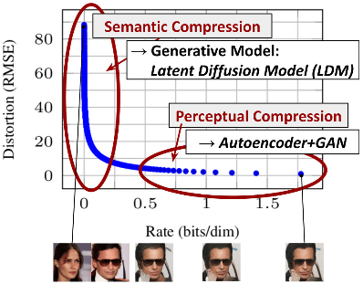
Figure 2. Illustrating perceptual and semantic compression: Most bits of a digital image correspond to imperceptible details. While DMs allow to suppress this semantically meaningless information by minimizing the responsible loss term, gradients (during training) and the neural network backbone (training and inference) still need to be evaluated on all pixels, leading to superfluous computations and unnecessarily expensive optimization and inference. We propose latent diffusion models (LDMs) as an effective generative model and a separate mild compression stage that only eliminates imperceptible details. Data and images from [27].
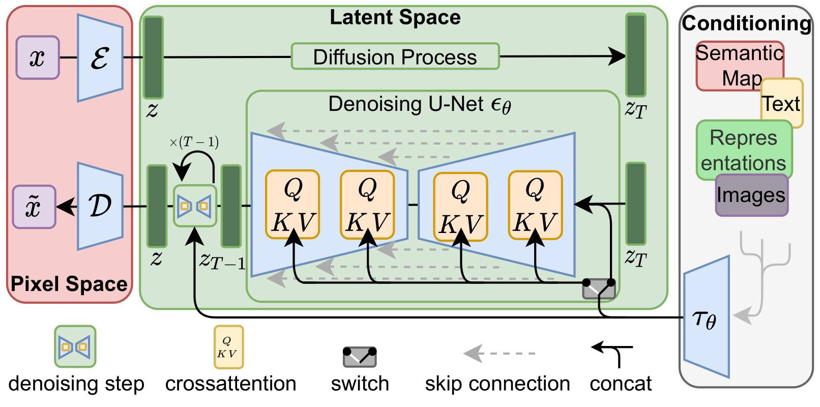
Figure 3. We condition LDMs either via concatenation or by a more general cross-attention mechanism. See Sec. 3.3
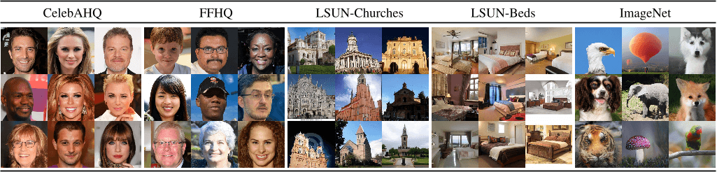
Figure 4. Samples from LDMs trained on CelebAHQ [35], FFHQ [37], LSUN-Churches [95], LSUN-Bedrooms [95] and class-conditional ImageNet [11], each with a resolution of 256× 256. Best viewed when zoomed in. For more samples cf . the supplement.
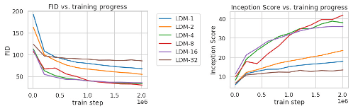
Figure 5. Analyzing the training of class-conditional LDMs with different downsampling factors f over 2M train steps on the ImageNet dataset. Pixel-based LDM-1 requires substantially larger train times compared to models with larger downsampling factors (LDM--12). Too much perceptual compression as in LDM-32 limits the overall sample quality. All models are trained on a single NVIDIA A100 with the same computational budget. Results obtained with 100 DDIM steps [79] and κ = 0.
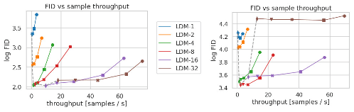
Figure 6. Inference speed vs sample quality: Comparing LDMs with different amounts of compression on the CelebA-HQ (left) and ImageNet (right) datasets. Different markers indicate 200 sampling steps with the DDIM sampler, counted from right to left along each line. The dashed line shows the FID scores for 200 steps, indicating the strong performance of LDM--4 compared to models with different compression ratios. FID scores assessed on 5000 samples. All models were trained for 500k (CelebA) / 2M (ImageNet) steps on an A100.
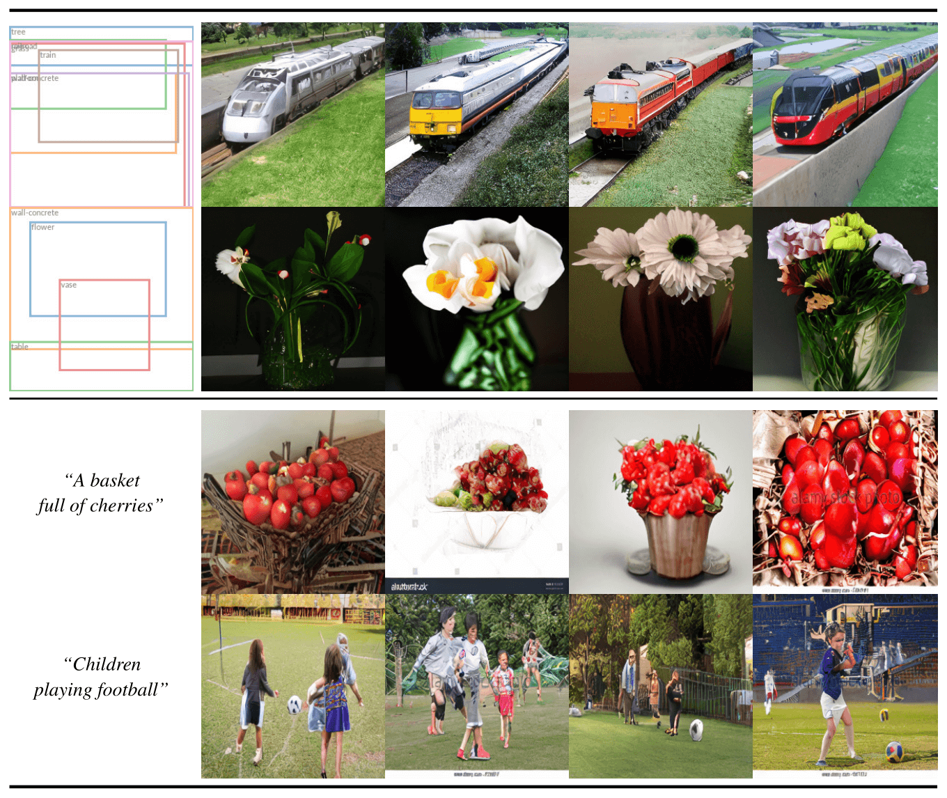
Figure 7. Top: Samples from our LDM for layout-to-image synthesis on COCO [4]. Quantitative evaluation in the supplement. Bottom: Samples from our text-to-image LDM for user-defined text prompts. Our model is pretrained on the LAION [73] database and finetuned on the Conceptual Captions [74] dataset.
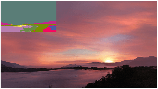
Figure 8. A LDM trained on 2562 resolution can generalize to larger resolution (here: 512×1024) for spatially conditioned tasks such as semantic synthesis of landscape images. See Sec. 4.3.2.
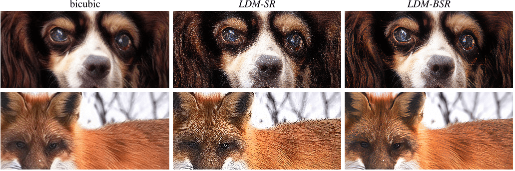
Figure 9. LDM-BSR generalizes to arbitrary inputs and can be used as a general-purpose upsampler, upscaling samples from a classconditional LDM (image cf . Fig. 4) to 10242 resolution. In contrast, using a fixed degradation process (see Sec. 4.4) hinders generalization.
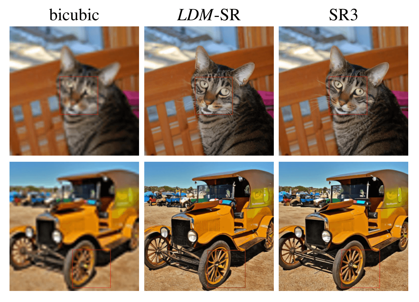
Figure 10. ImageNet 64→256 super-resolution on ImageNet-Val. LDM-SR has advantages at rendering realistic textures but SR3 can synthesize more coherent fine structures. See appendix for additional samples and cropouts. SR3 results from [67].
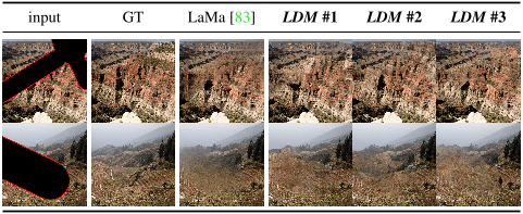
Figure 11. Qualitative results on image inpainting as in Tab. 6.
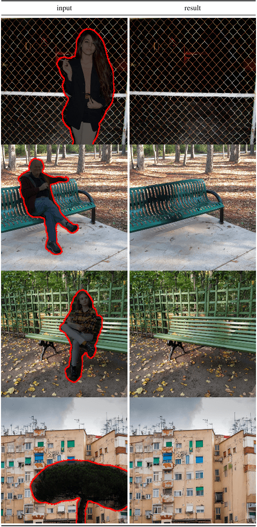
Figure 12. Qualitative results on object removal with our big, w/ ft inpainting model. For more results, see Fig. 22.
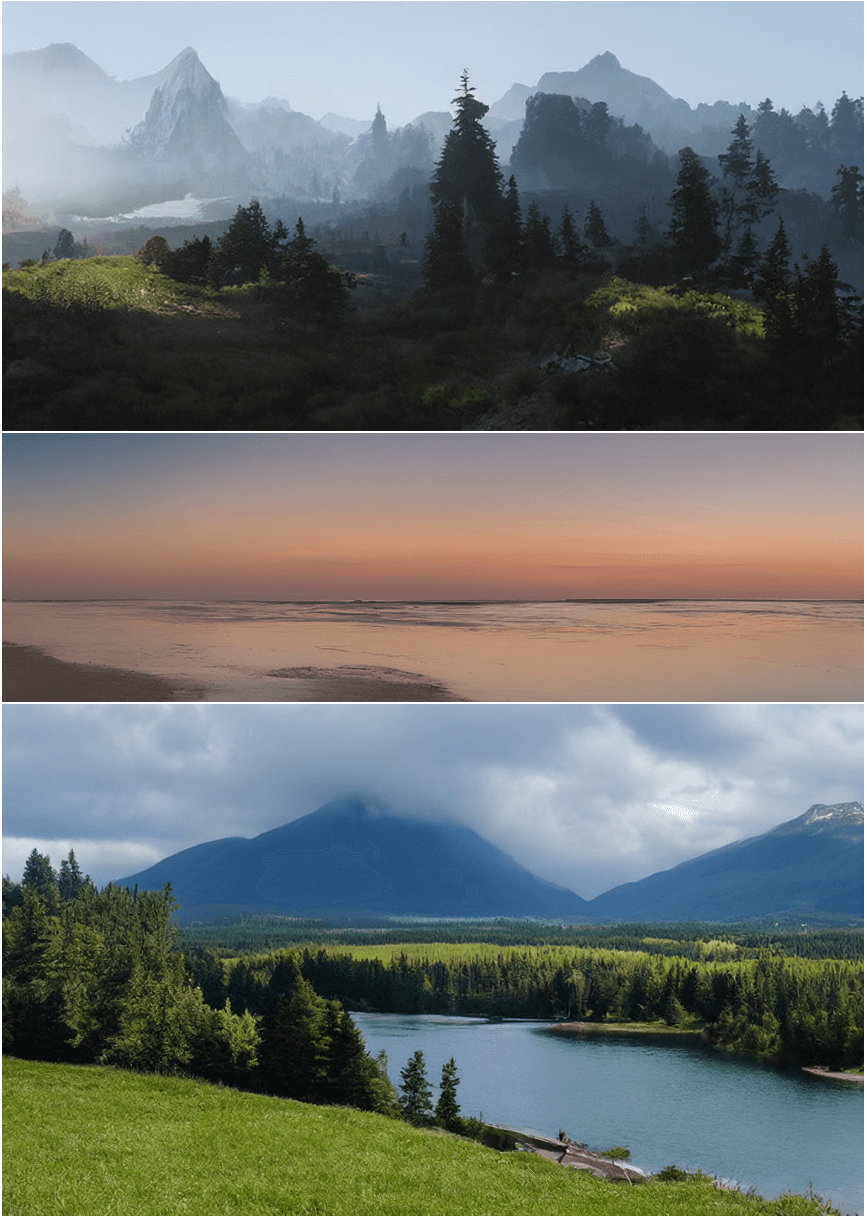
Figure 13. Convolutional samples from the semantic landscapes model as in Sec. 4.3.2, finetuned on 5122 images.
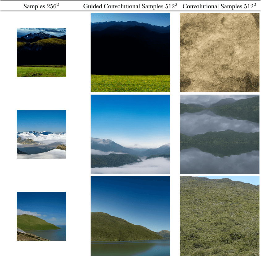
Figure 14. On landscapes, convolutional sampling with unconditional models can lead to homogeneous and incoherent global structures (see column 2). L2-guiding with a low resolution image can help to reestablish coherent global structures.
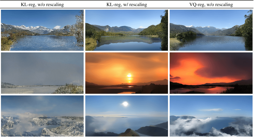
Figure 15. Illustrating the effect of latent space rescaling on convolutional sampling, here for semantic image synthesis on landscapes. See Sec. 4.3.2 and Sec. C.1.
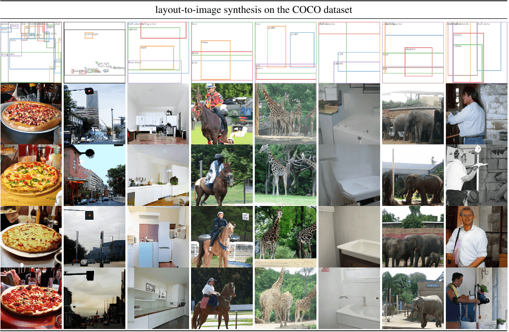
Figure 16. More samples from our best model for layout-to-image synthesis, LDM-4, which was trained on the OpenImages dataset and finetuned on the COCO dataset. Samples generated with 100 DDIM steps and η = 0. Layouts are from the COCO validation set.
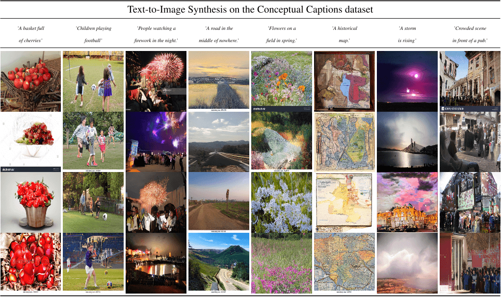
Figure 17. More samples for user-defined text prompts from our best model for Text-to-Image Synthesis, LDM-4, which was trained on the LAION database and finetuned on the Conceptual Captions dataset. Samples generated with 100 DDIM steps and η = 0.
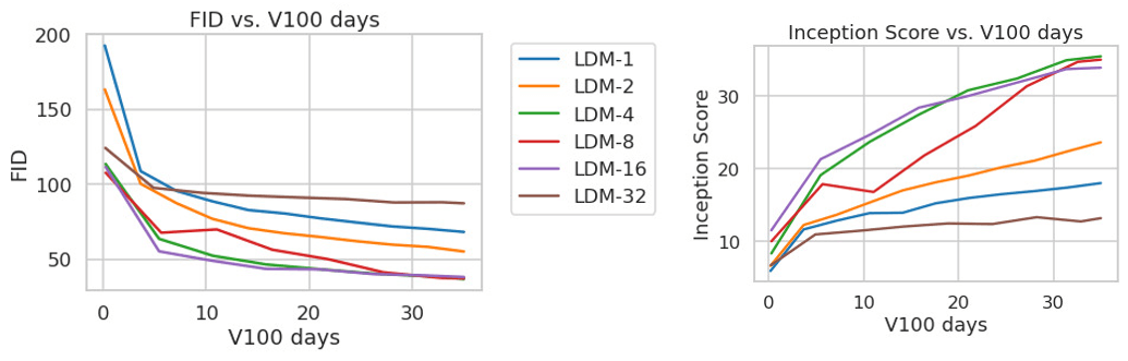
Figure 18. For completeness we also report the training progress of class-conditional LDMs on the ImageNet dataset for a fixed number of 35 V100 days. Results obtained with 100 DDIM steps [79] and κ = 0. FIDs computed on 5000 samples for efficiency reasons.
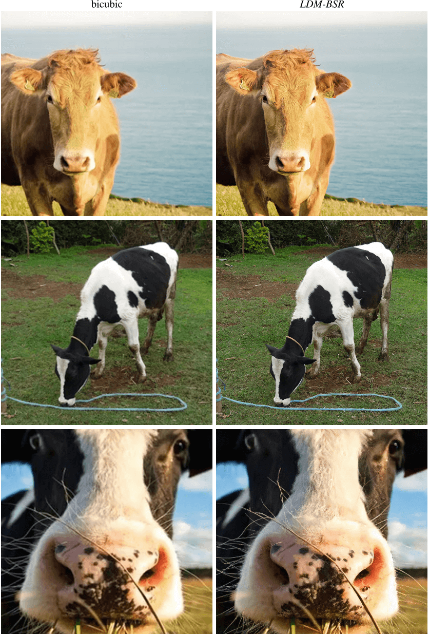
Figure 19. LDM-BSR generalizes to arbitrary inputs and can be used as a general-purpose upsampler, upscaling samples from the LSUNCows dataset to 10242 resolution.
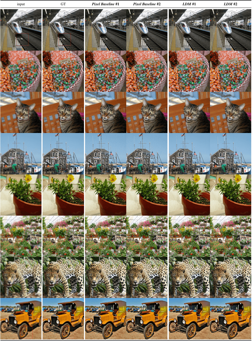
Figure 20. Qualitative superresolution comparison of two random samples between LDM-SR and baseline-diffusionmodel in Pixelspace. Evaluated on imagenet validation-set after same amount of training steps.
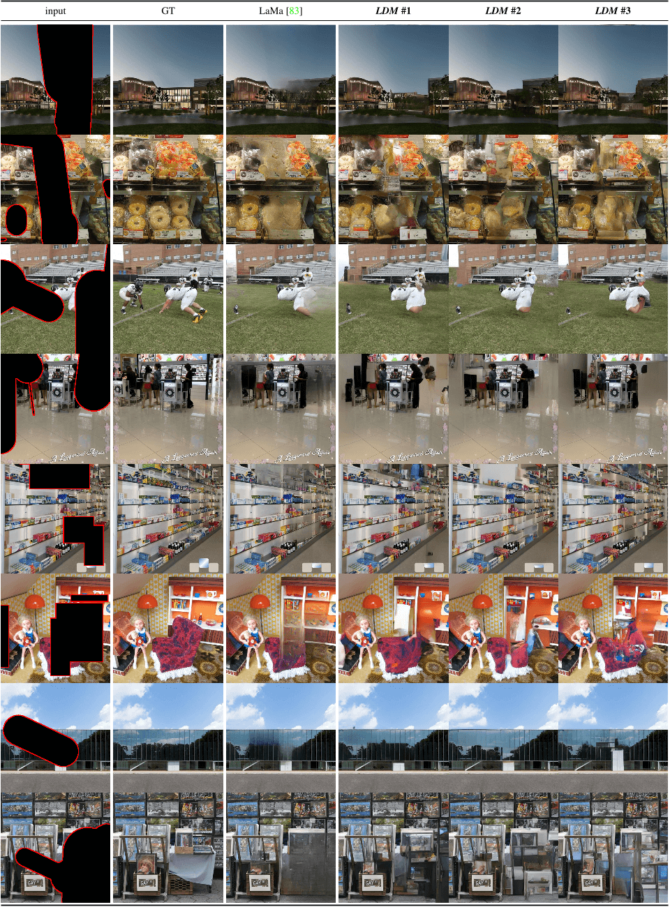
Figure 21. More qualitative results on image inpainting as in Fig. 11.
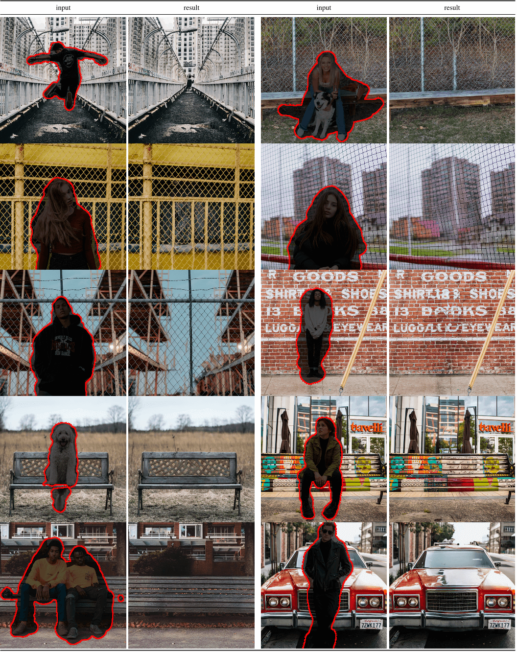
Figure 22. More qualitative results on object removal as in Fig. 12.
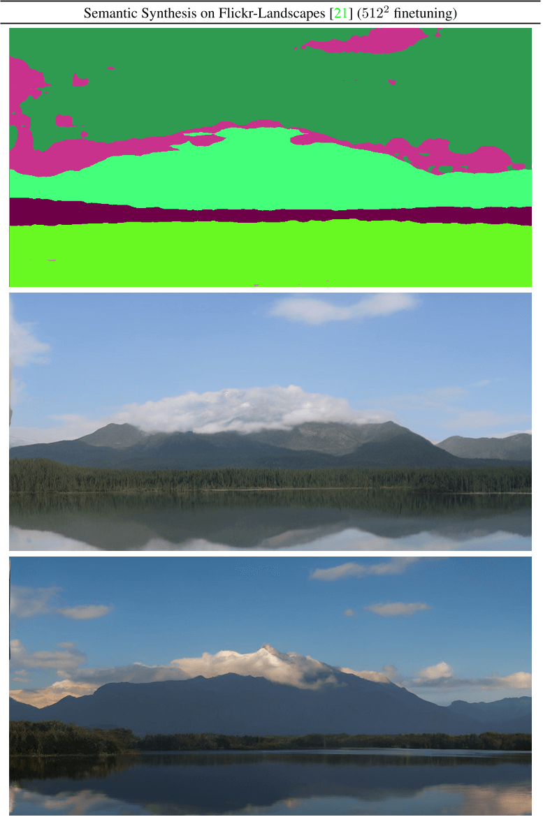
Figure 23. Convolutional samples from the semantic landscapes model as in Sec. 4.3.2, finetuned on 5122 images.
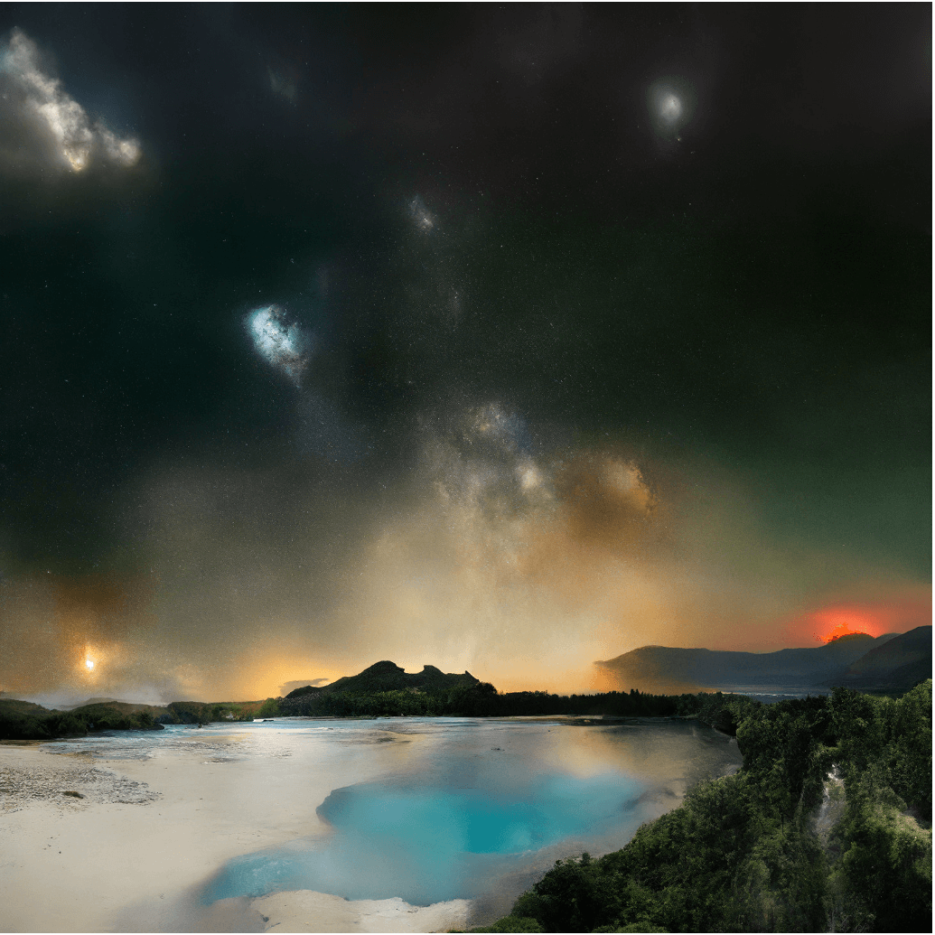
Figure 24. A LDM trained on 2562 resolution can generalize to larger resolution for spatially conditioned tasks such as semantic synthesis of landscape images. See Sec. 4.3.2.
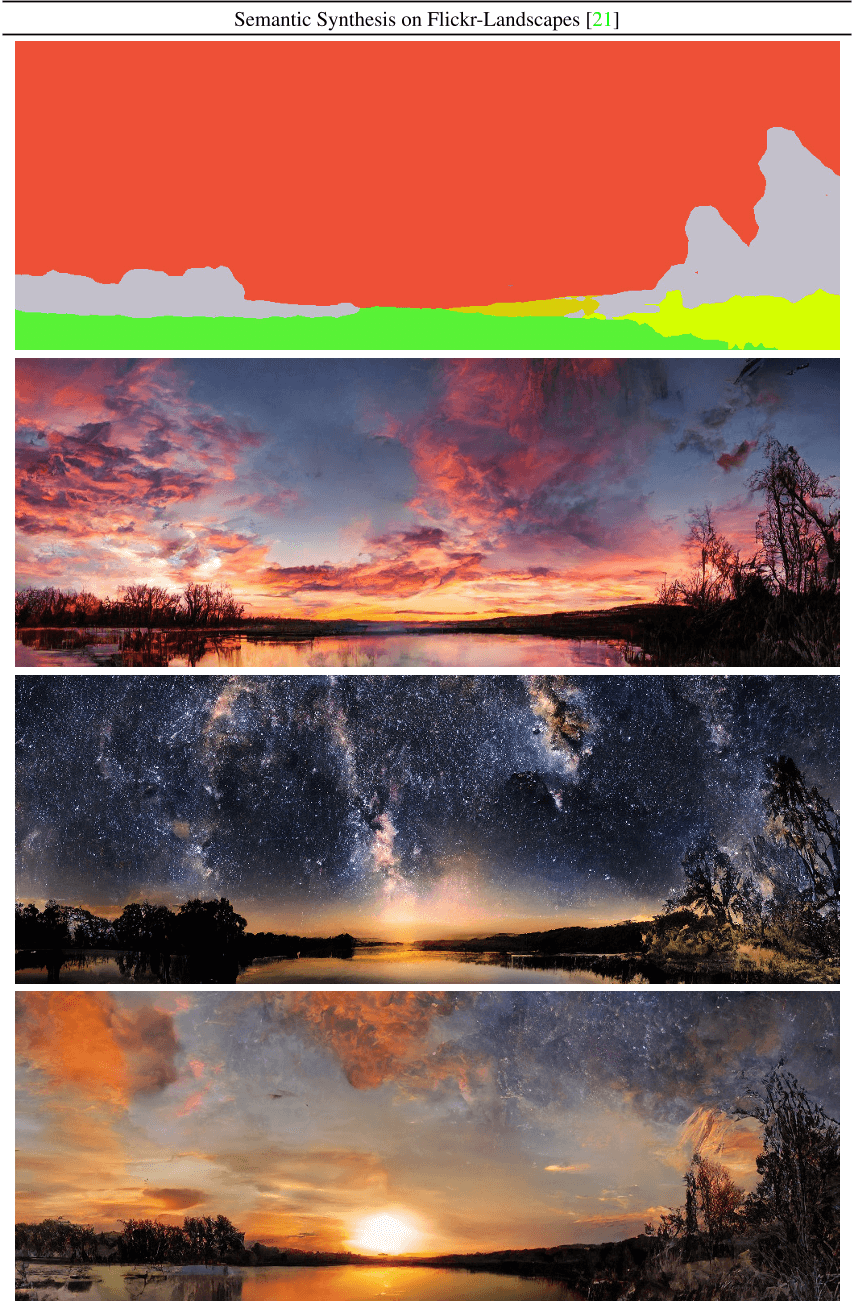
Figure 25. When provided a semantic map as conditioning, our LDMs generalize to substantially larger resolutions than those seen during training. Although this model was trained on inputs of size 2562 it can be used to create high-resolution samples as the ones shown here, which are of resolution 1024× 384. 31
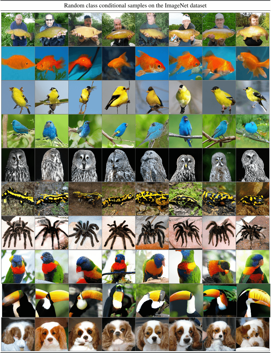
Figure 26. Random samples from LDM-8-G on the ImageNet dataset. Sampled with classifier scale [14] 50 and 100 DDIM steps with η = 1. (FID 8.5).
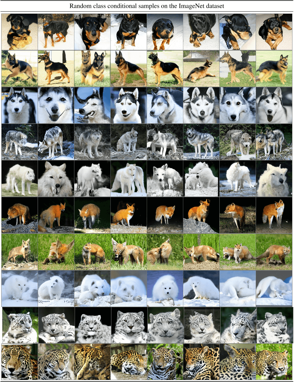
Figure 27. Random samples from LDM-8-G on the ImageNet dataset. Sampled with classifier scale [14] 50 and 100 DDIM steps with η = 1. (FID 8.5).
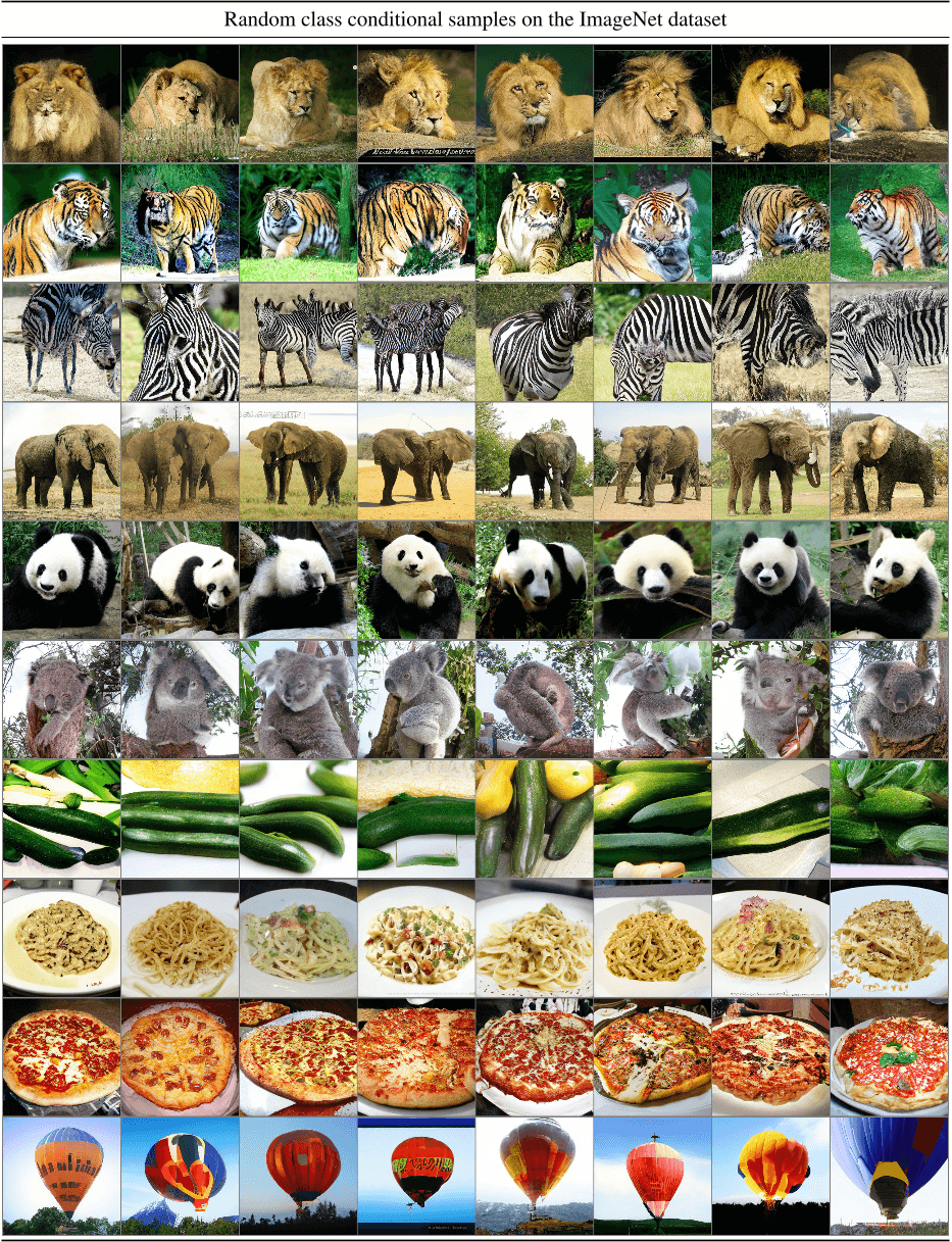
Figure 28. Random samples from LDM-8-G on the ImageNet dataset. Sampled with classifier scale [14] 50 and 100 DDIM steps with η = 1. (FID 8.5).
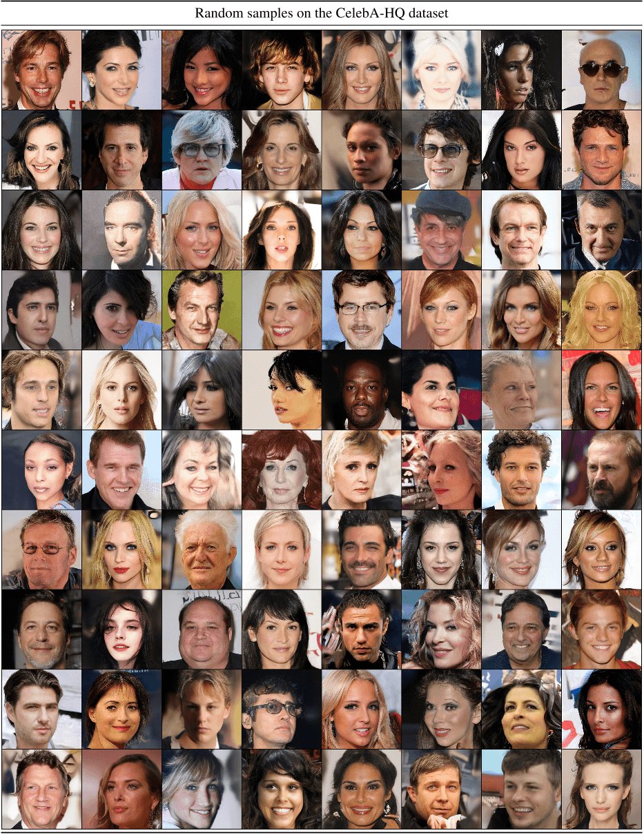
Figure 29. Random samples of our best performing model LDM-4 on the CelebA-HQ dataset. Sampled with 500 DDIM steps and η = 0 (FID = 5.15).
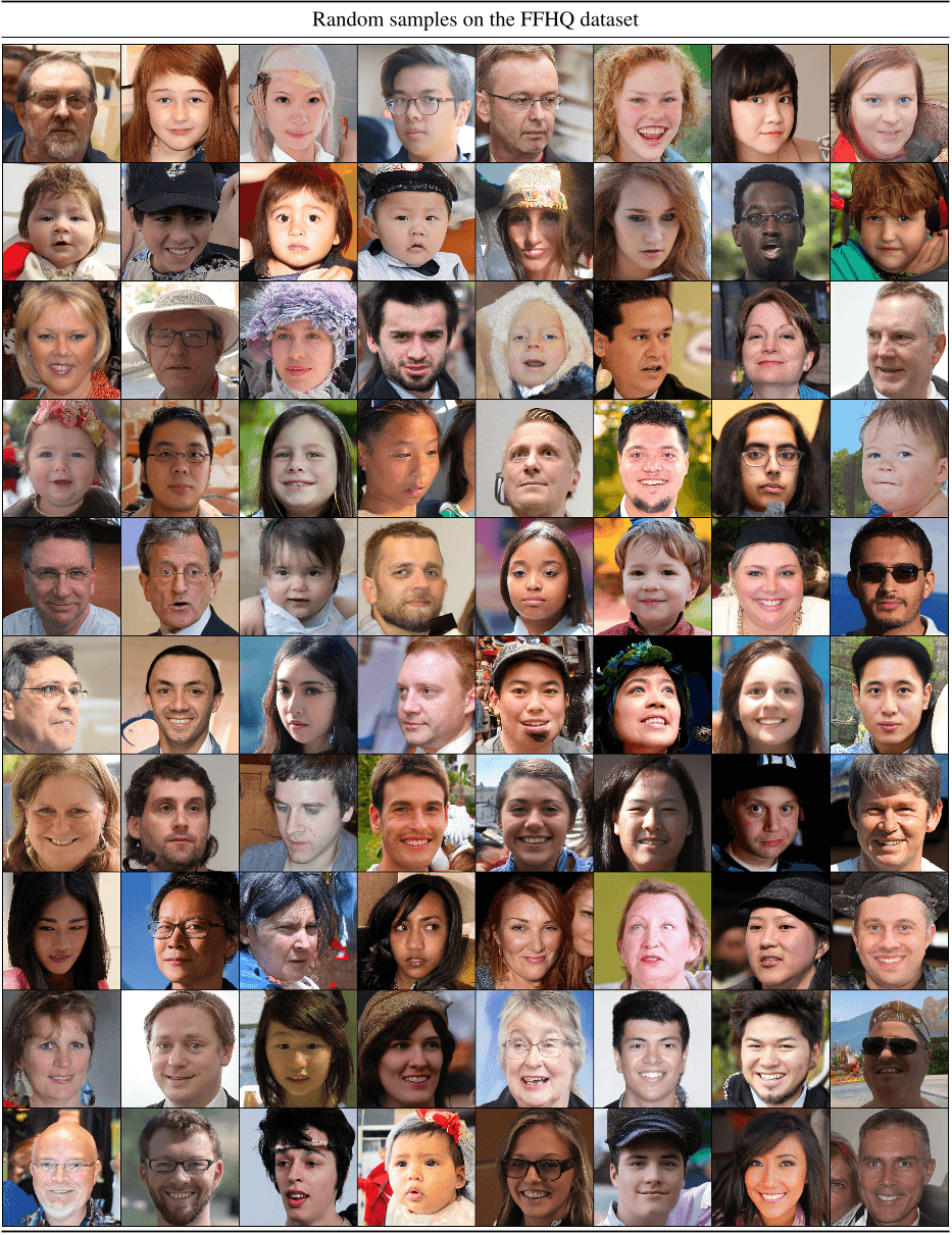
Figure 30. Random samples of our best performing model LDM-4 on the FFHQ dataset. Sampled with 200 DDIM steps and η = 1 (FID = 4.98).
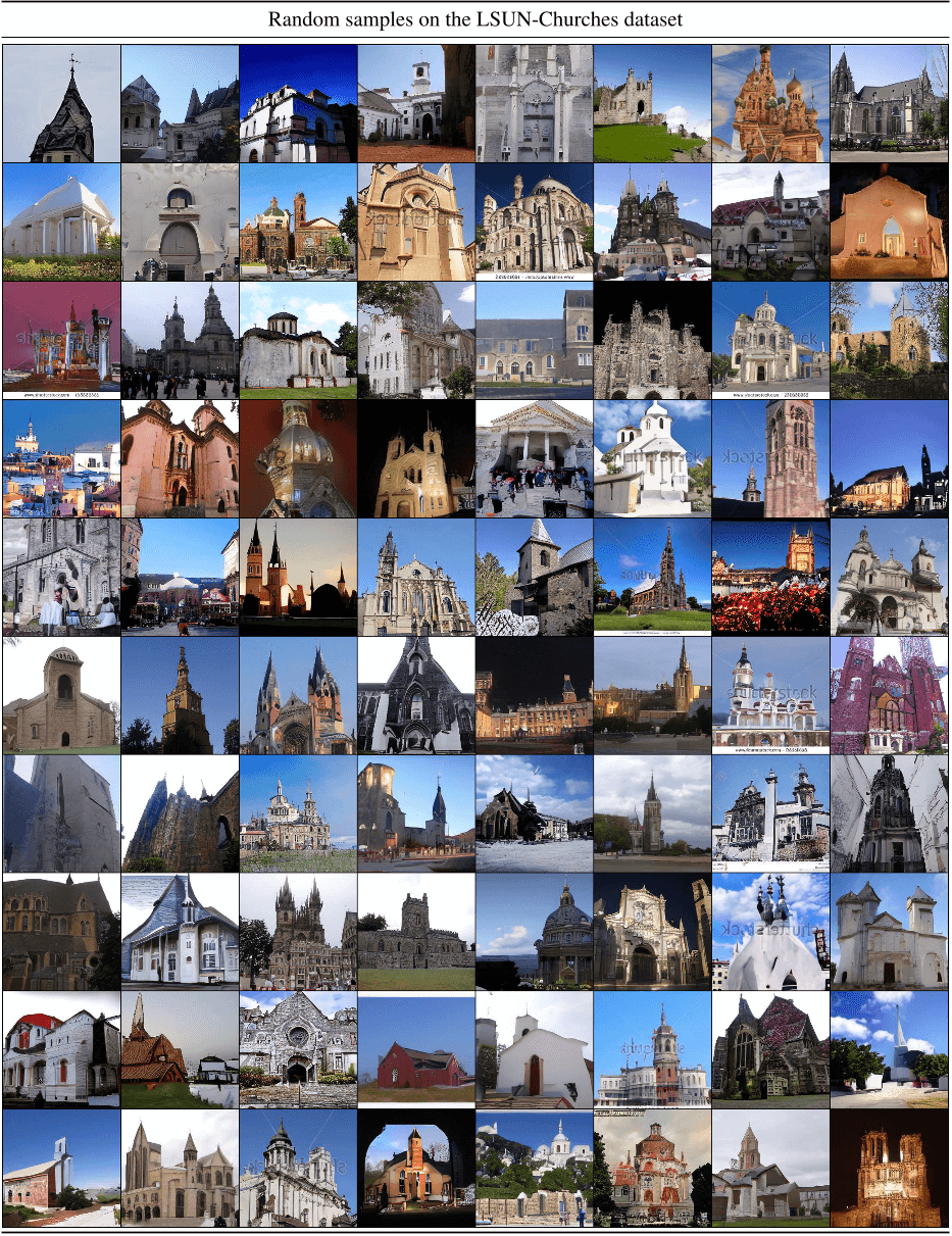
Figure 31. Random samples of our best performing model LDM-8 on the LSUN-Churches dataset. Sampled with 200 DDIM steps and η = 0 (FID = 4.48).
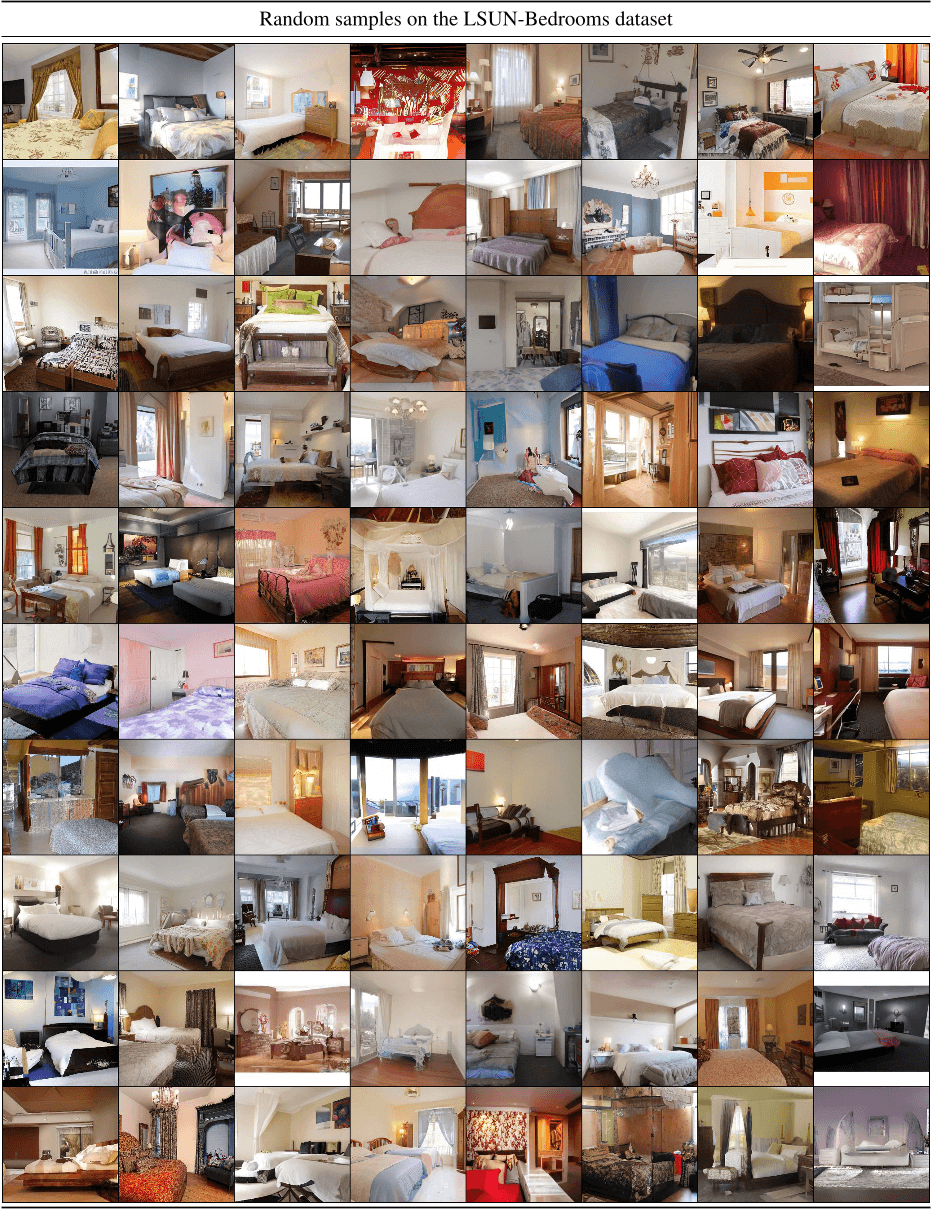
Figure 32. Random samples of our best performing model LDM-4 on the LSUN-Bedrooms dataset. Sampled with 200 DDIM steps and η = 1 (FID = 2.95).
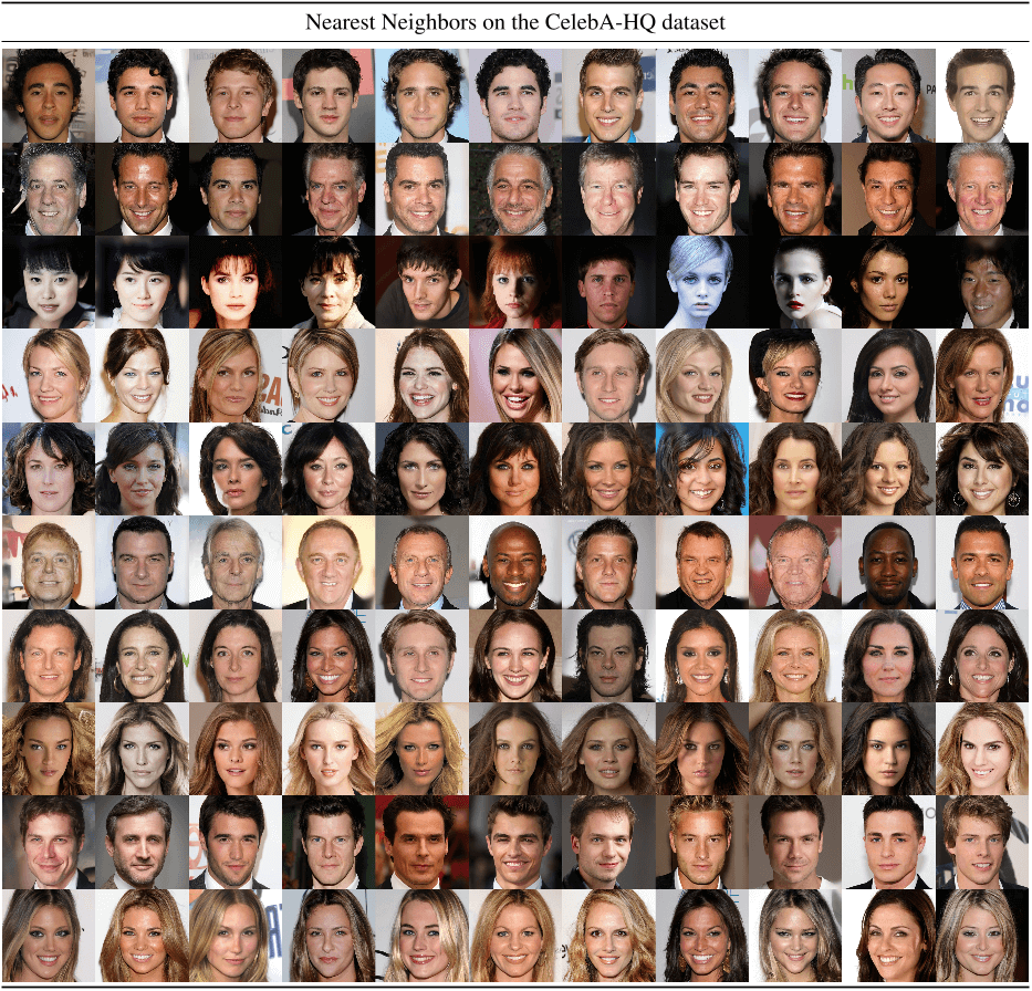
Figure 33. Nearest neighbors of our best CelebA-HQ model, computed in the feature space of a VGG-16 [75]. The leftmost sample is from our model. The remaining samples in each row are its 10 nearest neighbors.
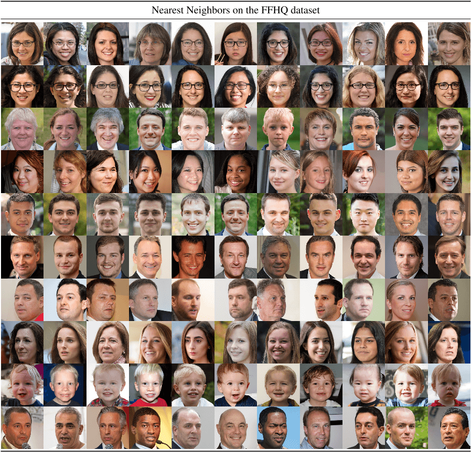
Figure 34. Nearest neighbors of our best FFHQ model, computed in the feature space of a VGG-16 [75]. The leftmost sample is from our model. The remaining samples in each row are its 10 nearest neighbors.
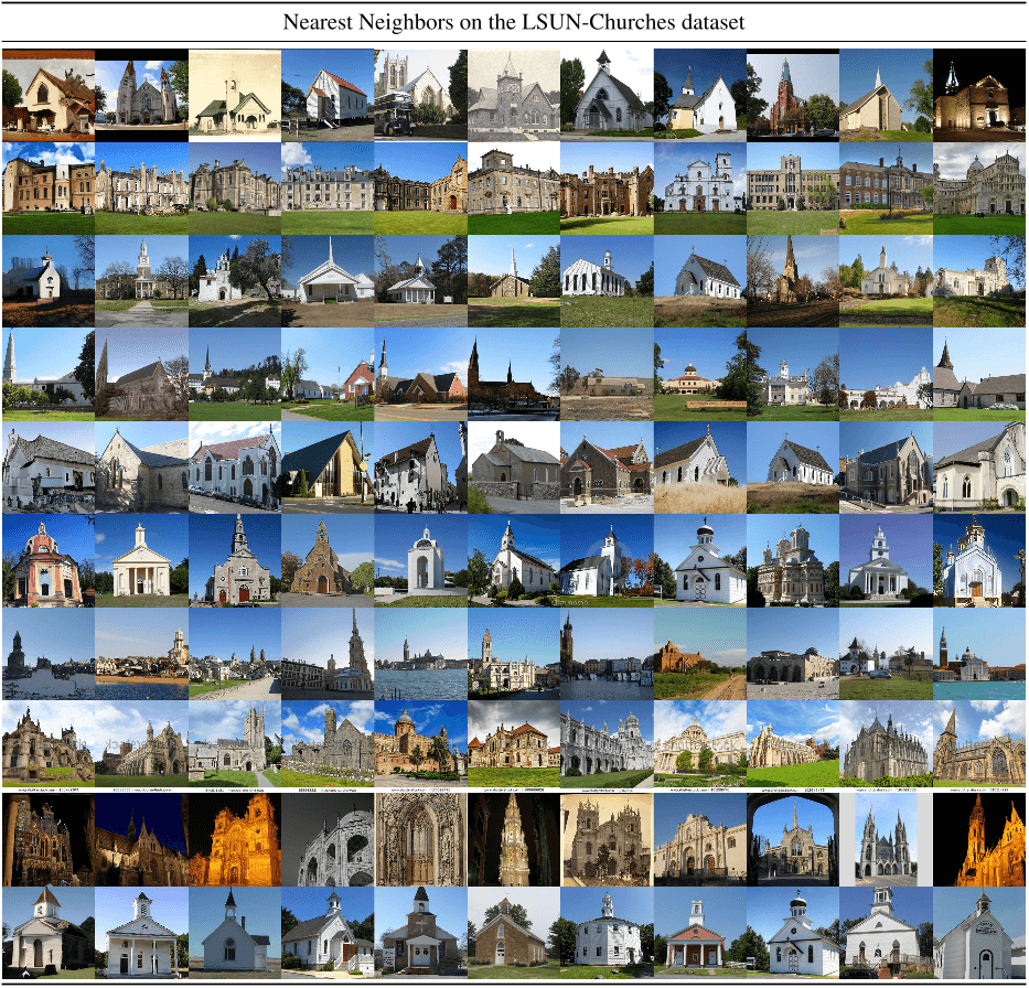
Figure 35. Nearest neighbors of our best LSUN-Churches model, computed in the feature space of a VGG-16 [75]. The leftmost sample is from our model. The remaining samples in each row are its 10 nearest neighbors.